Notation 

We use the following notation:

• \(N\) number of assets or securities in the universe (scalar)
• \(w\) is the column vector of weights (\(  N \times 1 \))
• \( \varSigma \) is the covariance matrix of returns, a positive definite matrix \( ( N \times N\))
• \(r_{p}\) is the expected return of a portfolio (scalar)
• \(r\)  is the vector of expected returns (\(  N \times 1 \))
• \(e\) the vector of ones (\(  N \times 1 \))
• \( r_{f} \) the risk free rate (scalar)

Mean-Variance optimisation

The standard mean variance portfolio selection model of [Markowitz (1952)] is based on the trade-off between return and risk and addresses the investor's asset selection problem for an investment horizon of one period.

The classical optimisation procedure for, a desired level of expected return, is given by:

\begin{eqnarray*} & \underset{w}{\text{minimize}} & & \sigma_{W}^{2}=  w^{'}\varSigma w\\ & \text{subject to} & & r_{p} =t  \\ & & & w^{'} e =1 \end{eqnarray*}

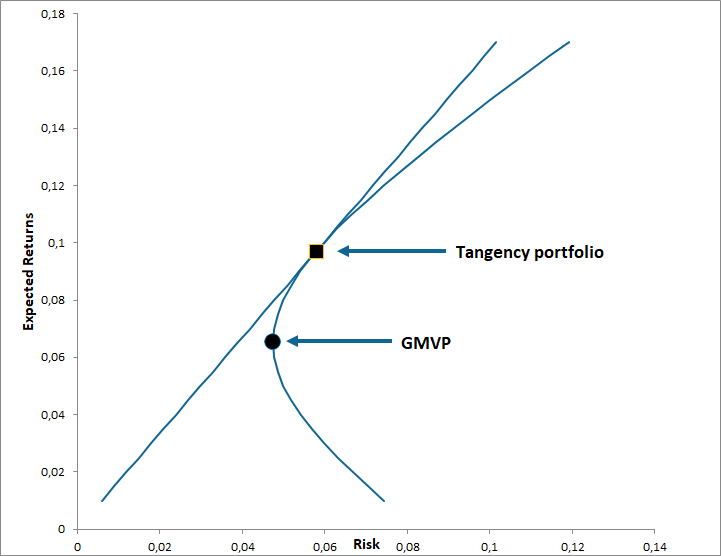
The portfolio mean, denoted \(r_{p} \) is given by : \(r_{p} =w^{'} r \) and its variance is given by \(\sigma_{p}^{2}= w^{'}\varSigma w > 0\). The volatility of the portfolio \(\sigma_{p} \) can be obtained via the function PORT.RISK. In this problem, we minimize the portfolio variance subject to the constraints: the portfolio weights must sum to unity and the portfolio must earn an expected rate of return equal to  \(t \). The set of portfolios that solve this problem (having the lowest variance for a given return) and that are located above the global minimum variance portfolio are called mean-variance efficient portfolios. The efficient frontier dominates all other investments in the opportunity set.  In mean-standard-deviation space, the efficient frontier is a hyperbola as shown in the following figure.

 

Alternatively, the same optimisation can be expressed in terms of a target variance such as: 

\begin{eqnarray*} & \underset{w}{\text{maximize}} & & r_{p}  = w^{'} r_{p} \\ & \text{subject to} & &  \sigma_{p}^{2}= t  \\ & & & w^{'} e =1 \end{eqnarray*}

Here, we maximise the mean of the portfolio with respect to a target variance. So the set of portfolios obtained also correspond to the efficient frontier.

A third option is to write an objective function which is a combination of the expected return and the risk.  An additional risk-averse parameter is included and rests on the Utility theory. XlQuant implements the following quadratic utility function :

\begin{eqnarray*} \underset{w}{\text{max}} & & w^{'} R - \dfrac{\lambda}{2} w^{'}\varSigma w \end{eqnarray*}

The greater the \( \lambda \) , the more risk averse the investor is.

If the investor can allocate wealth to a risk-free asset (i.e unlimited risk-free borrowing and lending at the risk-free rate), the new efficient frontier is a straight line (called the capital market line), starting at the risk-free point and tangent to the efficient frontier. In this case, the return of the portfolio is \( r_{p}^{*}=w^{'} r +(1-w^{'}e) r_{f}  =r_{f}  +w^{'} (r - e r_{f})  \).

 

The global minimum variance portfolio (GMVP) is the portfolio with the smallest possible variance for any mean return. It can be obtained via the function  GMVP. The tangency portfolio is the portfolio of risky assets on the efficient frontier at the point where the capital market line is tangent to the efficiency frontier. It can be retrieved using the function  TANGENT.PORT .

The three previously optimisation problems can easily be estimated via XlQuant. Some of them can be tuned by the use of additional constraints presented hereafter.

Supported Constraints

In practice, constraints are generally imposed during optimisation. XlQuants supports a large number of constraints, they are presented below.

• The "Full Investment" (FI) constraint : \(w^{'} e =1  \). This is the most commonly use constraint, it simply imposes that the sum of the weights adds up to one.
• The "No Short Sell" (NS) constraint :  \(w_{i} \geq 0\) , in this case weights cannot take negative values. Thus short-selling is not allowed.
• The "No Borrowing" (NB) constraint  \(  (1-w^{'}e) \geq 0 \), it can only be imposed if a risk-free asset is added to the optimisation problem. It imposes that the percentage invested in the risk-free asset is positive.
• The "Box"(BOX) constraint: \(   l_{i} \leq w_{i} \leq u_{i} \) that imposes a lower and upper bound limit.
• The "Turnover" (TU) constraints the total absolute difference between the initial (\(w_{o}\)) and the final weights (\(w\)) is restricted to be less or equal to an upper bound. 
• The "Cardinality" (CA) constraint, that imposes a maximum number (\(K \)) of selected assets.
  This requires adding a binary variable \(b_{i}\) that takes the value 1 if stock \(i\) is selected and 0 otherwise, in the optimisation problem.   

 Constraints are easily recognized when calling functions thanks to the sufix (ex: FI, NS ..) of functions.

The following tables present all optimisations that are implemented with the corresponding functions.

Mean-Variance Utility Optimization

Function	Objectives	Constraints
MVU	max \(w^{'} r - \dfrac{\lambda}{2} w^{'}\varSigma w\)
MVU.FI	max \(w^{'} r - \dfrac{\lambda}{2} w^{'}\varSigma w\)	\(w^{'} e =1  \)
MVU.FI.NS	max \(w^{'} r - \dfrac{\lambda}{2} w^{'}\varSigma w\)	\(w^{'} e =1 ; w_{i} \geq 0 \)
MVU.FI.BOX	max \(w^{'} r - \dfrac{\lambda}{2} w^{'}\varSigma w\)	\(w^{'} e =1  ; l_{i} \leq w_{i} \leq u_{i} \)
MVU.FI.TU.NS	max \(w^{'} r - \dfrac{\lambda}{2} w^{'}\varSigma w\)	\(w^{'} e =1  ; w_{i} \geq 0 ; \sum_{i=1}^{N} | w_{i}-w_{i,o} | \leq u \)
MVU.FI.CA	max \(w^{'} r - \dfrac{\lambda}{2} w^{'}\varSigma w\)	\(w^{'} e =1  ; \sum_{i=1}^{N} b_{i} \leq K \)
MVU.FI.CA.NS	max \(w^{'} r - \dfrac{\lambda}{2} w^{'}\varSigma w\)	\(w^{'} e =1  ; w_{i} \geq 0 ; \sum_{i=1}^{N} b_{i} \leq K \)

 

Optimal weights for a given risk

Function	Objectives	Constraints
MV.VOL.FI	max \( r_{p}\)	\(w^{'} e =1 ; \sigma^{2}_{p} = t\)
MV.VOL.FI.NS	max \( r_{p}\)	\(w^{'} e =1 ; w_{i} \geq 0 ; \sigma^{2}_{p} \leq t \)
MV.VOL.RF	max \( r_{p}^{*}\)	\(   \sigma^{2}_{p} = t \)

Optimal weights for a given return

Function	Objectives	Constraints
MV.RET.FI	min \( \sigma^{2}_{p}\)	\(w^{'} e =1; r_{p} =  t\)
MV.RET.FI.NS	min \( \sigma^{2}_{p}\)	\(w^{'} e =1 ; w_{i} \geq 0 ; r_{p} = t\)
MV.RET.RF	min \( \sigma^{2}_{p}\)	\( r_{p}^{*} = t \)

Black-Litterman Model

The Black-Litterman asset allocation [Black (1992)]model assumes that the returns of assets have a normal distribution with \( \mu \) being the expected return and \(  \varSigma \) the covariance matrix. That is [He (2005)]:

\begin{equation} \label{eq:bl1}  r \sim N(\mu, \varSigma ) \end{equation}

where \( r \) is the \(N\)-vector of asset returns. A key feature in this model is that the expected return,  \( \mu \), is treated as a random variable :

\begin{equation*}\mu  \sim N( \pi ,  \tau \varSigma )\end{equation*}

where \(  \pi  \)  is the equilibrium risk premium and \( \tau \) is a scalar indicting the uncertainty of the CAPM prior.  

In addition, this model permits the investor to have a number of views on the market returns. The investor's view are expressed via the following relation:

\begin{equation*} P \mu  = q+ \epsilon  \qquad \epsilon  \sim N(0,\Omega) \end{equation*}

where \(P\) is a \( K \times N \) matrix of views and \( q \) is a  \( K \)-vector of the expected returns on these views.

The BL model combines investors views and the market information to obtain the posterior distribution of the expected returns : \( N( \bar{\mu} , \bar{M}^{-1} ) \) where the mean and covariance are given by :

\begin{equation} \label{eq:blm}
E\left( \mu\right) = \bar{\mu} = \left[ (\tau \Sigma)^{-1} +   P^{T} \Omega^{-1} P  \right]^{-1}  \left[ (\tau \Sigma)^{-1} \pi +  P^{T} \Omega^{-1} q \right]
\end{equation}

and
\begin{equation}   \label{eq:blcov}
\sigma^{2}_{\mu} = \bar{M}^{-1}= \left[ (\tau \Sigma)^{-1} +   P^{T} \Omega^{-1} P  \right]^{-1}
\end{equation}

 

According to equation \eqref{eq:bl1} , \eqref{eq:blm} and  \eqref{eq:blcov}, the (combined) return distribution can be re-expressed as:

\begin{equation}  r \sim N(  \bar{\mu} ,\bar{\Sigma}) \end{equation}

where \(\bar{\Sigma} =\Sigma +\bar{M}^{-1}  \).

 

Two functions are available to compute the posterior expected mean \eqref{eq:blm} , and posterior covariance matrix  \eqref{eq:blcov}  :

• The posterior mean \( \bar{\mu} \) can be obtained via : BL.MEAN
• The posterior covariance \( \bar{M}^{-1}  \) via : BL.COV

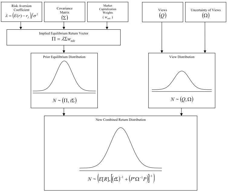
The whole model has nicely been summarised by T. Idzorek in the following figure.

Figure: "Deriving the New Combined Return Vector" from [Idzorek (2007)].

Risk Budgeting

The risk budgeting approach "is the analysis of the portfolio in terms of risk contributions rather than in term of portfolio weights" ([Maillard (2009)]). It decomposes a measure of portfolio risk into contributions from the individual assets in the portfolio. XlQuant uses the volatility of the portfolio as the risk measure.

The "Marginal Contribution to Risk" is the change in the total risk of the portfolio induced by an infinitesimal increase in holdings of component \(i\) and is formally defined by :

\begin{equation*} MCR_{k \times 1} = \frac{\partial \sigma_{p}}{\partial w} \end{equation*}

where  \(\sigma_{p}\) and  \(w\) are, respectively, the volatility of the portfolio and the vector of weights.

The "Contributions to Risk" are defined as the weighted marginal contributions:

\begin{equation*}CR_{i} = w_{i} \times MCR_{i} \end{equation*}

Alternatively, we may present the latter in percentages, by dividing the contribution to risk by the risk of the portfolio to obtain the "Percent Contribution to Risk".

 The "risk parity" or "Equally-weighted Risk Contribution" (ERC) portfolio is the portfolio where assets have equal risk contributions and is defined as ([Maillard (2009)]):

\begin{equation*}
 \left\lbrace  w^{*} =   w\in [0,1]^{n} : \sum w_{i} =1, w_{i} \times MCR_{i}   = w_{j} \times MCR_{j} \qquad \forall i,j    \right\rbrace
\end{equation*}

XlQuant provides several functions to apply these approach:

• MCTR : returns the Marginal Contribution to Risk.
• PCTR : returns the Percentage Contribution to Risk.
• CTR : returns the Contribution to Risk.
• ERC.FI : returns the Equally-weighted Risk Contribution portfolio with the Full Investment constraint.

Value-at-Risk and C-VaR

The Value-At-Risk metric is widely used to manage portfolio risk. The Basel Committee on Banking Supervision adopted the VaR methodology to measure market risk.

VaR is the maximum expected loss that will not be exceeded, at a given level of confidence, over a predetermined horizon. The formal definition of VaR, for a given return \(X\) is:

\begin{equation*}P(X < - VaR_{\alpha}) = \alpha \end{equation*}

The significance level \( \alpha \) corresponds to the confidence level \( 1- \alpha \). For instance, Basel II imposes VaR at the 1% significance level, i.e the 99% confidence level.

The Conditional-Var, measure the severity of the loss, given the loss is higher than the VaR, and is defined by:

\begin{equation*} CVaR_{\alpha}= -E(X | X < - VaR_{\alpha})  \end{equation*}

There exist three main methods to estimate these two metrics: the historical simulation, the parametric and the Monte-Carlo Method. XlQuant implements the historical and the parametric methods and assumes the portfolio is continually rebalanced so that the portfolio weights are constant.

Historical : This method simply infers the VaR and CVaR from the empirical distribution of returns (or prices). Therefore, by assuming constant weights, the VaR and CVaR are simply given by, respectively, the \(\alpha\) quantile of the history of the weighted returns and the average of the past returns bellow that quantile.

 

Parametric Linear : By assuming constant weights, a specific distribution of the factors (or returns) and Linear Risk factors, the VaR and C-VaR of a portfolio can be obtained analytically. XlQuant currently supports the Normal and Student distribution of factors.

The analytical formula implemented are [Alexander (2009)]:

Normal distribution:

 \begin{align*}
  VaR_{\alpha,h}(X)&=\left[ -h w' \mu + \sqrt{h}  \sqrt{ w \varSigma w'} \Phi^{-1}(1-\alpha)  \right]  P \\
 CVaR_{\alpha,h}(X) &=\left[ -h w' \mu + \sqrt{h}  \sqrt{ w \varSigma w'} \frac{ \phi( \Phi^{-1}(\alpha))}{\alpha}  \right]  P \end{align*}

where \(h\) is the horizon period, \(\alpha\) is the significant level, \(\mu\) the one-step expected (vector) returns, \(\Phi\) the CDF of the standard normal distribution and \(P\) is the value of the portfolio. Both equations are implemented in PORT.VaR.NORMAL and PORT.CVaR.NORMAL.

Student distribution:

 \begin{align*}
  VaR_{\alpha}(X)&=\left[ - w' \mu_{h} +   \sqrt{ \dfrac{v-2}{v}}  \sqrt{ w \varSigma_{h} w'} t^{-1}_{v}(1-\alpha) \right]   P\\
 CVaR_{\alpha}(X)&= \alpha^{-1} (v-1)^{-1}(v-2+x_{a}(v)^{2}) f_{v}(x_{a}(v)) \sigma_{h} - \mu_{h} 
 \end{align*}

where \(f_{v}\) denotes the standardized Student t density function and \(v\) the degrees of freedom. These equations are implemented in PORT.VaR.STUDENT and PORT.CVaR.STUDENT.

Miscellaneous

Measure of diversification:

• The Diversification Ratio, proposed by [Choueifaty (2008)] can be obtained via the function D.RATIO. It is defined as the ratio of its weighted average volatility and its volatility:

\begin{equation*}
  DR = \dfrac{w' \varSigma }{\sqrt{w \varSigma w'}}
\end{equation*}

• The volatility-weighted Concentration Ratio, proposed by the same authors can be obtained via the function C.RATIO. It is defined as:

\begin{equation*}
  CR =  \dfrac{\sum_{i = 1}^{N} (w_i \sigma_i)^2}{(\sum_{i = 1}^{N} w_i \sigma_i)^2}
 \end{equation*}

List of functions

BL.COV	Returns the (posterior) covariance matrix of the Black-Litterman master formula
BL.MEAN	Returns the (posterior) mean of the Black-Litterman master formula
C.RATIO	Returns the concentration ratio
CTR	Returns the contribution to risk, using the volatility as a risk measure
D.RATIO	Returns the diversification ratio
ERC.FI	Returns the equally-weighted risk contribution portfolio
GMVP	Calculates the global minimum portfolio
MCTR	Returns the marginal contribution to risk, using the volatility as a risk measure
MV.RET.FI	Calculates the optimum investments weights in a portfolio.
MV.RET.FI.NS	Calculates the optimum investments weights in a portfolio (without short sales).
MV.RET.RF	Calculates the optimum investments weights in a portfolio with a risk free asset
MV.VOL.FI	Calculates the optimum investments weights in a portfolio for a given volatility
MV.VOL.FI.NS	Calculates the optimum investments weights in a portfolio for a given volatility, without short sales
MV.VOL.RF	Calculates the optimum investments weights in a portfolio for a given volatility and risk free rate
MV.VOL.RF.NS	Calculates the optimum investments weights in a portfolio for a given volatility and risk free rate, without short sales
MV.VOL.RF.NS.NB	Calculates the optimum investments weights in a portfolio for a given volatility and risk free rate, without short sales and borrowing
MVU	MVU optimisation without constraint
MVU.FI	MVU optimisation with the full investment constraint
MVU.FI.BOX	MVU optimization with the full investment and bounds constraints
MVU.FI.CA	MVU optimisation with the full investment and the cardinality constraints
MVU.FI.NS	MVU optimisation with the full investment and long only constraints
MVU.FI.NS.CA	MVU optimisation with the full investment, long only and the cardinality constraints
MVU.FI.TU.NS	MVU optimisation with : the full investment, long only and the turnover constraints.
PCTR	Returns the percentage contribution to risk, using the volatility as a risk measure
PORT.CVaR	Returns the historical CVaR of a portfolio
PORT.CVaR.NORMAL	Returns the Conditional Value-At-Risk of a Normal Linear Model
PORT.CVaR.STUDENT	Returns the Conditional Value-At-Risk of a Student-t Linear Model
PORT.RISK	Returns the volatility of a portfolio.
PORT.VaR	Returns the historical VaR of a portfolio
PORT.VaR.NORMAL	Returns the Value-At-Risk of a Normal Linear Model
PORT.VaR.STUDENT	Returns the Value-At-Risk of a Student-t Linear Model
TANGENT.PORT	Calculates the tangent portfolio

Bibliography

• Markowitz H. Portfolio Selection. J Finance. 1952;7(1):77-91.

• Choueifaty Y, Coignard Y. Toward Maximum Diversification. The Journal of Portfolio Management. 2008.

• B. O'Donoghue and E. Chu and N. Parikh and S. Boyd. Conic Optimization via Operator Splitting and Homogeneous Self-Dual Embedding. Journal of Optimization Theory and Applications 2016

• Maillard S, Roncalli T, Teiletche J. On the Properties of Equally-Weighted Risk Contributions Portfolios.; 2009.

• Alexander C. Market Risk Analysis Volume IV - Value-at-Risk Models. John Wiley and Sons Ltd; 2009

• He G, Litterman R. The Intuition Behind Black-Litterman Model Portfolios. SSRN Electron J. 2005.

• Thomas Idzorek ;A step-by-step guide to the Black–Litterman model in Forecasting Expected Returns in the Financial Markets; Edited by Stephen Satchell, Elsevier, 2007

• Boyd S, Vandenberghe L. Convex Optimization. Cambridge University Press; 2009.

• Black F, Litterman R. Global Portfolio Optimization. Financ Anal J. 1992;48(5).